Getting Started with Mint
This section presents a complete code walk-through of an example Mint
application, designed to illustrate some of the key concepts and capabilities
of Mint. The complete Mint Application Code Example, is included in the
Appendix section and is also available in the Axom source
code under src/axom/mint/examples/user_guide/mint_getting_started.cpp.
The example Mint application demonstrates how Mint is used to develop kernels that are both mesh-agnostic and device-agnostic.
Tip
Mint’s RAJA-based Execution Model helps facilitate the implementation of various computational kernels that are both mesh-agnostic and device-agnostic. Both kernels discussed in this example do not make any assumptions about the underlying mesh type or the target execution device, e.g. CPU or GPU. Consequently, the same implementation can operate on both Structured Mesh and Unstructured Mesh types and run sequentially or in parallel on all execution devices supported through RAJA.
Prerequisites
Understanding the discussion and material presented in this section requires:
Working knowledge of C++ templates and Lambda Expression functions.
High-level understanding of nested memory hierarchies on heterogeneous architectures and CUDA Unified Memory.
Basics of the Execution Model (recommended)
Note
Mint does not provide a memory manager. The application must explicitly specify the desired allocation strategy and memory space to use. This is facilitated by using Umpire for memory management. Specifically, this example uses CUDA Unified Memory when compiled with RAJA and CUDA enabled by setting the default Umpire allocator in the beginning of the program as follows:
  // NOTE: use unified memory if we are using CUDA or HIP
  const int allocID = axom::execution_space<ExecPolicy>::allocatorID();
  axom::setDefaultAllocator(allocID);
When Umpire , RAJA and CUDA are not enabled, the code will use the
malloc() internally to allocate memory on the host and all kernels will
be executed on the CPU.
Goals
Completion of the walk-though of this simple code example should only require a few minutes. Upon completion, the user will be familiar with using Mint to:
Create and evaluate fields on a mesh
Use the Node Traversal Functions and Cell Traversal Functions of the Execution Model to implement kernels that operate on the mesh and associated fields.
Plot the mesh and associated fields in VTK for visualization.
Step 1: Add Header Includes
First, the Mint header must be included for the definition of the various Mint classes and functions. Note, this example also makes use of Axom’s Matrix class, which is also included by the following:
1#include "axom/config.hpp"                          // compile time definitions
2#include "axom/core/execution/execution_space.hpp"  // for execution_space traits
3
4#include "axom/mint.hpp"                  // for mint classes and functions
5#include "axom/core/numerics/Matrix.hpp"  // for numerics::Matrix
Step 2: Get a Mesh
The example application is designed to operate on either a Structured Mesh or an Unstructured Mesh. The type of mesh to use is specified by a runtime option that can be set by the user at the command line. See Step 7: Run the Example for more details.
To make the code work with both Structured Mesh and Unstructured Mesh
instances the kernels are developed in terms of the The Mesh Base Class,
mint::Mesh.
The pointer to a mint::Mesh object is acquired as follows:
1 mint::Mesh* mesh = (Arguments.useUnstructured) ? getUnstructuredMesh() : getUniformMesh();
When using a Uniform Mesh, the mesh is constructed by the following:
1mint::Mesh* getUniformMesh()
2{
3  // construct a N x N grid within a domain defined in [-5.0, 5.0]
4  const double lo[] = {-5.0, -5.0};
5  const double hi[] = {5.0, 5.0};
6  mint::Mesh* m = new mint::UniformMesh(lo, hi, Arguments.res, Arguments.res);
7  return m;
8}
This creates an \(N \times N\) Uniform Mesh, defined on a domain given by the interval \(\mathcal{I}:[-5.0,5.0] \times [-5.0,5.0]\), where \(N=25\), unless specified otherwise by the user at the command line.
When an Unstructured Mesh is used, the code will generate the Uniform Mesh internally and triangulate it by subdividing each quadrilateral element into four triangles. See the complete Mint Application Code Example for details.
See the Tutorial for more details on how to Create a Uniform Mesh or Create an Unstructured Mesh.
Step 3: Add Fields
Fields are added to the mesh by calling the createField() method
on the mesh object:
1  // add a cell-centered and a node-centered field
2  double* phi = mesh->createField<double>("phi", mint::NODE_CENTERED);
3  double* hc = mesh->createField<double>("hc", mint::CELL_CENTERED);
4
5  constexpr int NUM_COMPONENTS = 2;
6  double* xc = mesh->createField<double>("xc", mint::CELL_CENTERED, NUM_COMPONENTS);
The node-centered field,
phi, stores the result, computed in Step 4: Evaluate a Scalar FieldThe cell-centered field,
hc, stores the nodal average ofphi, computed in Step 5: Average to Cell CentersThe cell-centered field,
xc, stores the cell-centers, computed in Step 5: Average to Cell Centers
Note, the template argument to the createField() method indicates the
underlying field type, e.g. double, int , etc. In this case, all three
fields have a double field type.
The first required argument to the createField() method is a string
corresponding to the name of the field. The second argument, which is also
required, indicates the centering of the field, i.e. node-centered,
cell-centered or face-centered.
A third, optional, argument may be specified to indicate the number of
components of the corresponding field. In this case, the node-centered field,
phi, is a scalar field. However, the cell-centered field, xc,
is a 2D vector quantity, which is specified explicitly by
supplying the third argument in the createField() method invocation.
Note
Absence of the third argument when calling createField() indicates
that the number of components of the field defaults to \(1\) and thereby
the field is assumed to be a scalar quantity.
See the Tutorial for more details on Working with Fields on a mesh.
Step 4: Evaluate a Scalar Field
The first kernel employs the for_all_nodes() traversal function of the
Execution Model to iterate over the constituent
mesh Nodes and evaluate Himmelblau’s Function at each node:
 1  // loop over the nodes and evaluate Himmelblaus Function
 2  mint::for_all_nodes<ExecPolicy, xargs::xy>(
 3    mesh,
 4    AXOM_LAMBDA(IndexType nodeIdx, double x, double y) {
 5      const double x_2 = x * x;
 6      const double y_2 = y * y;
 7      const double A = x_2 + y - 11.0;
 8      const double B = x + y_2 - 7.0;
 9
10      phi[nodeIdx] = A * A + B * B;
11    });
The arguments to the
for_all_nodes()function consists of:A pointer to the mesh object, and
The kernel that defines the per-node operations, encapsulated within a Lambda Expression, using the convenience AXOM_LAMBDA Macro.
In addition, the
for_all_nodes()function has two template arguments:ExecPolicy: The execution policy specifies, where and how the kernel is executed. It is a required template argument that corresponds to an Execution Policy defined by the Execution Model.xargs::xy: Indicates that in addition to the index of the node,nodeIdx, the kernel takes thexandynode coordinates as additional arguments.
Within the body of the kernel, Himmelblau’s Function is evaluated using the
supplied x and y node coordinates. The result is stored in the
corresponding field array, phi, which is captured by the
Lambda Expression, at the corresponding node location, phi[ nodeIdx ].
See the Tutorial for more details on using the Node Traversal Functions of the Execution Model.
Step 5: Average to Cell Centers
The second kernel employs the for_all_cells() traversal function of the
Execution Model to iterate over the constituent mesh
Cells and performs the following:
computes the corresponding cell centroid, a 2D vector quantity,
averages the node-centered field,
phi, computed in Step 4: Evaluate a Scalar Field, at the cell center.
 1  // loop over cells and compute cell centers
 2  mint::for_all_cells<ExecPolicy, xargs::coords>(
 3    mesh,
 4    AXOM_LAMBDA(IndexType cellIdx, const numerics::Matrix<double>& coords, const IndexType* nodeIds) {
 5      // NOTE: A column vector of the coords matrix corresponds to a nodes coords
 6
 7      // Sum the cell's nodal coordinates
 8      double xsum = 0.0;
 9      double ysum = 0.0;
10      double hsum = 0.0;
11
12      const IndexType numNodes = coords.getNumColumns();
13      for(IndexType inode = 0; inode < numNodes; ++inode)
14      {
15        const double* node = coords.getColumn(inode);
16        xsum += node[mint::X_COORDINATE];
17        ysum += node[mint::Y_COORDINATE];
18
19        hsum += phi[nodeIds[inode]];
20      }  // END for all cell nodes
21
22      // compute cell centroid by averaging the nodal coordinate sums
23      const IndexType offset = cellIdx * NUM_COMPONENTS;
24      const double invnnodes = 1.f / static_cast<double>(numNodes);
25      xc[offset] = xsum * invnnodes;
26      xc[offset + 1] = ysum * invnnodes;
27
28      hc[cellIdx] = hsum * invnnodes;
29    });
Similarly, the arguments to the
for_all_cells()function consists of:A pointer to the mesh object, and
The kernel that defines the per-cell operations, encapsulated within a Lambda Expression, using the convenience AXOM_LAMBDA Macro.
In addition, the
for_all_cells()function has two template arguments:ExecPolicy: As with thefor_all_nodes()function, the execution policy specifies, where and how the kernel is executed.xargs::coords: Indicates that in addition to the index of the cell,cellIdx, the supplied kernel takes two additional arguments:coords, a matrix that stores the node coordinates of the cell, andnodeIds, an array that stores the IDs of the constituent cell nodes.
The cell node coordinates matrix, defined by axom::numerics::Matrix is
organized such that:
The number of rows of the matrix corresponds to the cell dimension, and,
The number of columns of the matrix corresponds to the number of cell nodes.
The \(ith\) column vector of the matrix stores the coordinates of the \(ith\) cell node.
In this example, the 2D Uniform Mesh, consists of 2D rectangular cells,
which are defined by \(4\) nodes. Consequently, the supplied node coordinates
matrix to the kernel, coords, will be a \(2 \times 4\) matrix of the
following form:
Within the body of the kernel, the centroid of the cell is calculated by
averaging the node coordinates. The code loops over the columns of the
coords matrix (i.e., the cell nodes) and computes the sum of each
node coordinate in xsum and ysum respectively. Then, the average is
evaluated by multiplying each coordinate sum with \(1/N\), where \(N\)
is the number of nodes of a cell. The result is stored in the corresponding
field array, xc, which is captured by the Lambda Expression.
Since, the cell centroid is a 2D vector quantity, each cell entry has an
x-component and y-component. Multi-component fields in Mint are stored using a
2D row-major contiguous memory layout, where, the number of rows corresponds to
the number of cells, and the number of columns correspond to the number of
components of the field. Consequently, the x-component of the centroid of a cell
with ID, cellIdx is stored at xc[ cellIIdx * NUM_COMPONENTS ] and the
y-component is stored at xc[ cellIdx * NUM_COMPONENTS + 1 ], where
NUM_COMPONENTS=2.
In addition, the node-centered quantity, phi, computed in Step 4: Evaluate a Scalar Field is
averaged and stored at the cell centers. The kernel first sums all the nodal
contributions in hsum and then multiplies by \(1/N\), where \(N\)
is the number of nodes of a cell.
See the Tutorial for more details on using the Cell Traversal Functions of the Execution Model.
Step 6: Output the Mesh in VTK
Last, the resulting mesh and data can be output in the Legacy VTK File Format, which can be visualized by a variety of visualization tools, such as VisIt and ParaView as follows:
1  // write the mesh in a VTK file for visualization
2  std::string vtkfile = (Arguments.useUnstructured) ? "unstructured_mesh.vtk" : "uniform_mesh.vtk";
3  mint::write_vtk(mesh, vtkfile);
A VTK file corresponding to the VTK File Format specification for the mesh type used will be generated.
Step 7: Run the Example
After building the Axom Toolkit, the basic Mint example may be run from within the build space directory as follows:
> ./examples/mint_getting_started_ex
By default the example will use a \(25 \times 25\) Uniform Mesh domain
defined on the interval \(\mathcal{I}:[-5.0,5.0] \times [-5.0,5.0]\).
The resulting VTK file is stored in the specified file, uniform_mesh.vtk.
A depiction of the mesh showing a plot of Himmelblau’s Function computed
over the constituent Nodes of the mesh is illustrated in
Fig. 4.
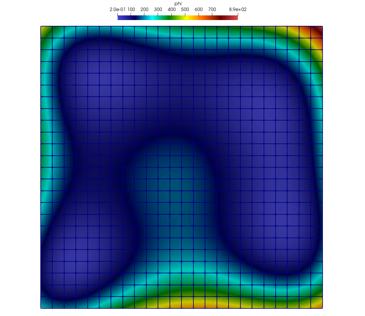
Fig. 4 Plot of Himmelblau’s Function computed over the constituent Nodes of the Uniform Mesh.
The user may choose to use an Unstructured Mesh instead by specifying
the --unstructured option at the command line as follows:
> ./examples/mint_getting_started_ex --unstructured
The code will generate an Unstructured Mesh by triangulating the
Uniform Mesh such that each quadrilateral is subdivided into four triangles.
The resulting unstructured mesh is stored in a VTK file, unstructured_mesh.vtk,
depicted in Fig. 5.
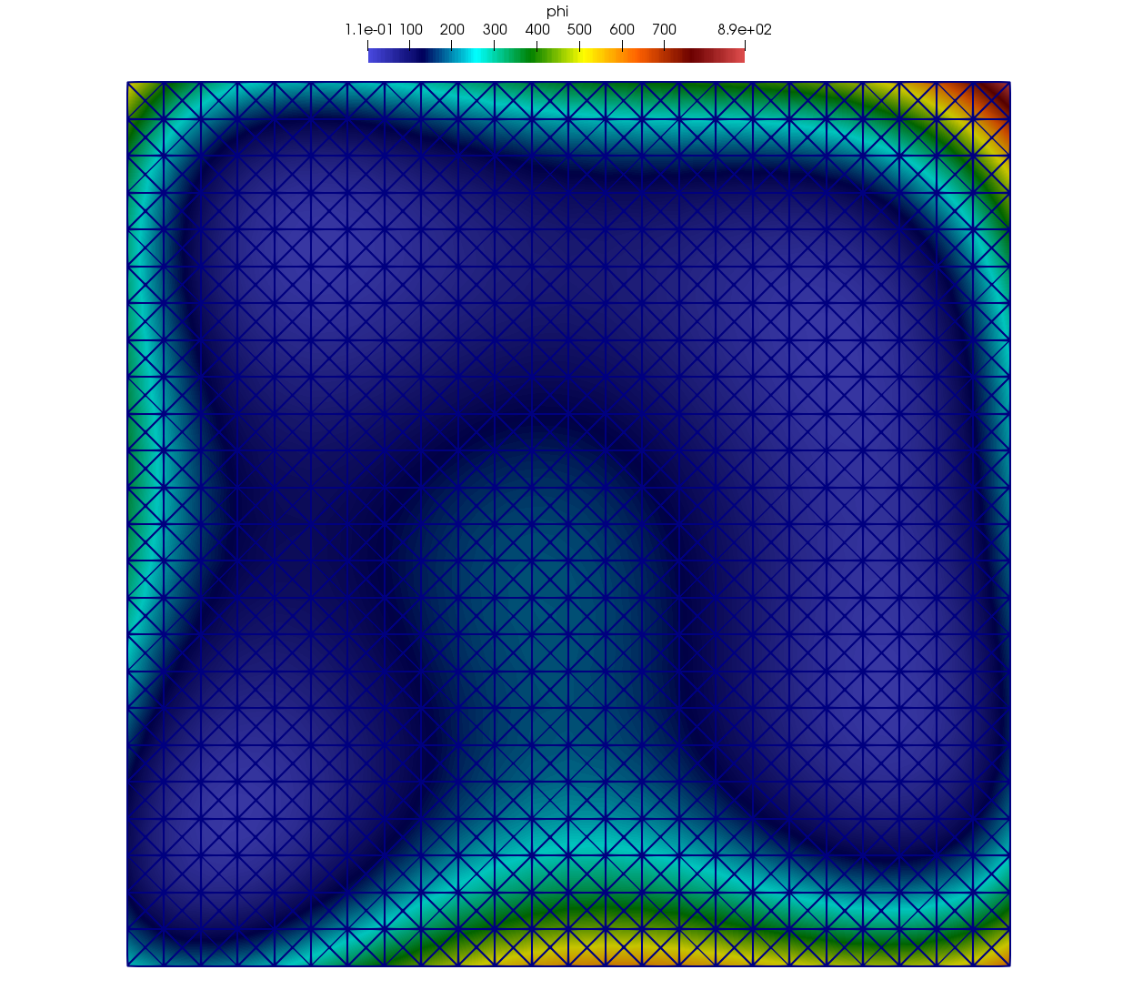
Fig. 5 Plot of Himmelblau’s Function computed over the constituent Nodes of the Unstructured Mesh.
By default the resolution of the mesh is set to \(25 \times 25\). A user
may set the desired resolution to use at the command line, using the
--resolution [N] command line option.
For example, the following indicates that a mesh of resolution \(100 \times 100\) will be used instead when running the example.
> ./examples/mint_getting_started_ex --resolution 100
Note
This example is designed to run:
In parallel on the GPU when the Axom Toolkit is compiled with RAJA and CUDA enabled.
In parallel on the CPU when the Axom Toolkit is compiled with RAJA and OpenMP enabled.
Sequentially on the CPU, otherwise.