Tutorial
The Tutorial section consists of simple examples and code snippets that illustrate how to use Mint’s core classes and functions to construct and operate on the various supported Mesh Types. The examples presented herein aim to illustrate specific Mint concepts and capabilities in a structured and simple format. To quickly learn basic Mint concepts and capabilities through an illustrative walk-through of a complete working code example, see the Getting Started with Mint section. Additional code examples, based on Mint mini-apps, are provided in the Examples section. For thorough documentation of the interfaces of the various classes and functions in Mint, developers are advised to consult the Mint Doxygen API Documentation, in conjunction with this Tutorial.
Create a Uniform Mesh
A Uniform Mesh is relatively the simplest Structured Mesh type, but also, the most restrictive mesh out of all Mesh Types. The constituent Nodes of the Uniform Mesh are uniformly spaced along each axis on a regular lattice. Consequently, a Uniform Mesh can be easily constructed by simply specifying the spatial extents of the domain and desired dimensions, e.g. the number of Nodes along each dimension.
For example, a \(50 \times 50\) Uniform Mesh, defined on a bounded domain given by the interval \(\mathcal{I}:[-5.0,5.0] \times [-5.0,5.0]\), can be easily constructed as follows:
1  const double lo[] = {-5.0, -5.0};
2  const double hi[] = {5.0, 5.0};
3  mint::UniformMesh mesh(lo, hi, 50, 50);
The resulting mesh is depicted in Fig. 25.

Fig. 25 Resulting Uniform Mesh.
Create a Rectilinear Mesh
A Rectilinear Mesh, also called a product mesh, is similar to a Uniform Mesh. However, the constituent Nodes of a Rectilinear Mesh are not uniformly spaced. The spacing between adjacent Nodes can vary arbitrarily along each axis, but the Topology of the mesh remains a regular Structured Mesh Topology. To allow for this flexibility, the coordinates of the Nodes along each axis are explicitly stored in separate arrays, i.e. \(x\), \(y\) and \(z\), for each coordinate axis respectively.
The following code snippet illustrates how to construct a \(25 \times 25\) Rectilinear Mesh where the spacing of the Nodes grows according to an exponential stretching function along the \(x\) and \(y\) axis respectively. The resulting mesh is depicted in Fig. 26.
 1  constexpr double beta = 0.1;
 2  const double expbeta = exp(beta);
 3  const double invf = 1 / (expbeta - 1.0);
 4
 5  // construct a N x N rectilinear mesh
 6  constexpr axom::IndexType N = 25;
 7  mint::RectilinearMesh mesh(N, N);
 8  double* x = mesh.getCoordinateArray(mint::X_COORDINATE);
 9  double* y = mesh.getCoordinateArray(mint::Y_COORDINATE);
10
11  // fill the coordinates along each axis
12  x[0] = y[0] = 0.0;
13  for(int i = 1; i < N; ++i)
14  {
15    const double delta = (exp(i * beta) - 1.0) * invf;
16    x[i] = x[i - 1] + delta;
17    y[i] = y[i - 1] + delta;
18  }
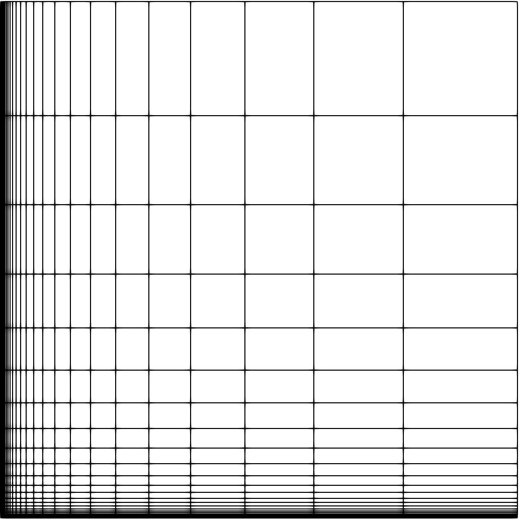
Fig. 26 Resulting Rectilinear Mesh.
Create a Curvilinear Mesh
A Curvilinear Mesh, also called a body-fitted mesh, is the most general of the Structured Mesh types. Similar to the Uniform Mesh and Rectilinear Mesh types, a Curvilinear Mesh also has regular Structured Mesh Topology. However, the coordinates of the Nodes comprising a Curvilinear Mesh are defined explicitly, enabling the use of a Structured Mesh discretization with more general geometric domains, i.e., the domain may not be necessarily Cartesian. Consequently, the coordinates of the Nodes are specified explicitly in separate arrays, \(x\), \(y\), and \(z\).
The following code snippet illustrates how to construct a \(25 \times 25\) Curvilinear Mesh. The coordinates of the Nodes follow from the equation of a cylinder with a radius of \(2.5\). The resulting mesh is depicted in Fig. 27.
 1  constexpr double R = 2.5;
 2  constexpr double M = (2 * M_PI) / 50.0;
 3  constexpr double h = 0.5;
 4  constexpr axom::IndexType N = 25;
 5
 6  // construct the curvilinear mesh object
 7  mint::CurvilinearMesh mesh(N, N);
 8
 9  // get a handle on the coordinate arrays
10  double* x = mesh.getCoordinateArray(mint::X_COORDINATE);
11  double* y = mesh.getCoordinateArray(mint::Y_COORDINATE);
12
13  // fill the coordinates of the curvilinear mesh
14  const axom::IndexType jp = mesh.nodeJp();
15  for(axom::IndexType j = 0; j < N; ++j)
16  {
17    const axom::IndexType j_offset = j * jp;
18
19    for(axom::IndexType i = 0; i < N; ++i)
20    {
21      const axom::IndexType nodeIdx = i + j_offset;
22
23      const double xx = h * i;
24      const double yy = h * j;
25      const double alpha = yy + R;
26      const double beta = xx * M;
27
28      x[nodeIdx] = alpha * cos(beta);
29      y[nodeIdx] = alpha * sin(beta);
30    }  // END for all i
31
32  }  // END for all j
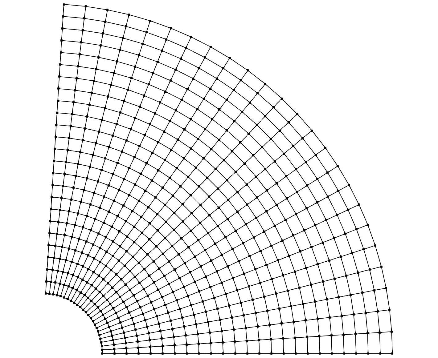
Fig. 27 Resulting Curvilinear Mesh.
Create an Unstructured Mesh
An Unstructured Mesh with Single Cell Type Topology has both explicit Topology and Geometry. However, the cell type that the mesh stores is known a priori, allowing for an optimized underlying Mesh Representation, compared to the more general Mixed Cell Type Topology Mesh Representation.
Since both Geometry and Topology are explicit, an Unstructured Mesh is created by specifying:
the coordinates of the constituent Nodes, and
the Cells comprising the mesh, defined by the cell-to-node Connectivity

Fig. 28 Resulting Single Cell Type Topology Unstructured Mesh
The following code snippet illustrates how to create the simple Unstructured Mesh depicted in Fig. 28.
 1  constexpr int DIMENSION = 2;
 2  constexpr mint::CellType CELL_TYPE = mint::TRIANGLE;
 3
 4  // Construct the mesh object
 5  mint::UnstructuredMesh<mint::SINGLE_SHAPE> mesh(DIMENSION, CELL_TYPE);
 6
 7  // Append the mesh nodes
 8  const axom::IndexType n0 = mesh.appendNode(0.0, 0.0);
 9  const axom::IndexType n1 = mesh.appendNode(2.0, 0.0);
10  const axom::IndexType n2 = mesh.appendNode(1.0, 1.0);
11  const axom::IndexType n3 = mesh.appendNode(3.5, 1.0);
12  const axom::IndexType n4 = mesh.appendNode(2.5, 2.0);
13  const axom::IndexType n5 = mesh.appendNode(5.0, 0.0);
14
15  // Append mesh cells
16  const axom::IndexType c0[] = {n1, n3, n2};
17  const axom::IndexType c1[] = {n2, n0, n1};
18  const axom::IndexType c2[] = {n3, n4, n2};
19  const axom::IndexType c3[] = {n1, n5, n3};
20
21  mesh.appendCell(c0);
22  mesh.appendCell(c1);
23  mesh.appendCell(c2);
24  mesh.appendCell(c3);
An Unstructured Mesh is represented by the mint::UnstructuredMesh
template class. The template argument of the class, mint::SINGLE_SHAPE
indicates the mesh has Single Cell Type Topology. The two arguments to the
class constructor correspond to the problem dimension and cell type, which
in this case, is \(2\) and mint::TRIANGLE respectively. Once the mesh
is constructed, the Nodes and Cells are appended to the mesh by
calls to the appendNode() and appendCell() methods respectively.
The resulting mesh is shown in Fig. 28.
Tip
The storage for the mint::UstructuredMesh will grow dynamically as new
Nodes and Cells are appended on the mesh. However, reallocations
tend to be costly operations. For best performance, it is advised the node
capacity and cell capacity for the mesh are specified in the constructor if
known a priori. Consult the Mint Doxygen API Documentation for more
details.
Create a Mixed Unstructured Mesh
Compared to the Single Cell Type Topology Unstructured Mesh, a Mixed Cell Type Topology Unstructured Mesh has also explicit Topology and Geometry. However, the cell type is not fixed. Notably, the mesh can store different Cell Types, e.g. triangles and quads, as shown in the simple 2D mesh depicted in Fig. 29.

Fig. 29 Sample Mixed Cell Type Topology Unstructured Mesh
As with the Single Cell Type Topology Unstructured Mesh, a Mixed Cell Type Topology Unstructured Mesh is created by specifying:
the coordinates of the constituent Nodes, and
the Cells comprising the mesh, defined by the cell-to-node Connectivity
The following code snippet illustrates how to create the simple Mixed Cell Type Topology Unstructured Mesh depicted in Fig. 29, consisting of \(2\) triangles and \(1\) quadrilateral Cells.
 1  constexpr int DIMENSION = 2;
 2
 3  // Construct the mesh object
 4  mint::UnstructuredMesh<mint::MIXED_SHAPE> mesh(DIMENSION);
 5
 6  // Append the mesh nodes
 7  const axom::IndexType n0 = mesh.appendNode(0.0, 0.0);
 8  const axom::IndexType n1 = mesh.appendNode(2.0, 0.0);
 9  const axom::IndexType n2 = mesh.appendNode(1.0, 1.0);
10  const axom::IndexType n3 = mesh.appendNode(3.5, 1.0);
11  const axom::IndexType n4 = mesh.appendNode(2.5, 2.0);
12  const axom::IndexType n5 = mesh.appendNode(5.0, 0.0);
13
14  // Append mesh cells
15  const axom::IndexType c0[] = {n0, n1, n2};
16  const axom::IndexType c1[] = {n1, n5, n3, n2};
17  const axom::IndexType c2[] = {n3, n4, n2};
18
19  mesh.appendCell(c0, mint::TRIANGLE);
20  mesh.appendCell(c1, mint::QUAD);
21  mesh.appendCell(c2, mint::TRIANGLE);
Similarly, a Mixed Cell Type Topology Unstructured Mesh is represented
by the mint::UnstructuredMesh template class. However, the template argument
to the class is mint::MIXED_SHAPE, which indicates that the mesh has
Mixed Cell Type Topology. In this case, the class constructor takes only a
single argument that corresponds to the problem dimension, i.e. \(2\).
Once the mesh is constructed, the constituent Nodes of the mesh are
specified by calling the appendNode() method on the mesh. Similarly, the
Cells are specified by calling the appendCell() method. However,
in this case, appendCell() takes one additional argument that specifies the
cell type, since that can vary.
Tip
The storage for the mint::UstructuredMesh will grow dynamically as new
Nodes and Cells are appended on the mesh. However, reallocations
tend to be costly operations. For best performance, it is advised the node
capacity and cell capacity for the mesh are specified in the constructor if
known a priori. Consult the Mint Doxygen API Documentation for more
details.
Working with Fields
A mesh typically has associated Field Data that store various numerical quantities on the constituent Nodes, Cells and Faces of the mesh.
Warning
Since a Particle Mesh is defined by a set of Nodes, it can only store Field Data at its constituent Nodes. All other supported Mesh Types can have Field Data associated with their constituent Cells, Faces and Nodes.
Add Fields
Given a mint::Mesh instance, a field is created by specifying:
The name of the field,
The field association, i.e. centering, and
Optionally, the number of components of the field, required if the field is not a scalar quantity.
For example, the following code snippet creates the scalar density field,
den, stored at the cell centers, and the vector velocity field, vel,
stored at the Nodes:
1    double* den = mesh->createField<double>("den", mint::CELL_CENTERED);
2    double* vel = mesh->createField<double>("vel", mint::NODE_CENTERED, 3);
Note
If Sidre is used as the backend Mesh Storage Management substrate,
createField() will populate the Sidre tree hierarchy accordingly.
See Using Sidre for more information.
Note, the template argument to the
createField()method indicates the underlying field type, e.g.double,int, etc. In this case, both fields are ofdoublefield type.The name of the field is specified by the first required argument to the
createField()call.The field association, is specified by the second argument to the
createField()call.A third, optional, argument may be specified to indicate the number of components of the corresponding field. In this case, since
velis a vector quantity the number of components must be explicitly specified.The
createField()method returns a raw pointer to the data corresponding to the new field, which can be used by the application.
Note
Absence of the third argument when calling createField() indicates
that the number of components of the field defaults to \(1\) and thereby
the field is assumed to be a scalar quantity.
Request Fields by Name
Specific, existing fields can be requested by calling getFieldPtr() on
the target mesh as follows:
1  double* den = mesh->getFieldPtr<double>("den", mint::CELL_CENTERED);
2
3  axom::IndexType nc = -1;  // number of components
4  double* vel = mesh->getFieldPtr<double>("vel", mint::NODE_CENTERED, nc);
As with the
createField()method, the template argument indicates the underlying field type, e.g.double,int, etc.The first argument specifies the name of the requested field
The second argument specifies the corresponding association of the requested field.
The third argument is optional and it can be used to get back the number of components of the field, i.e. if the field is not a scalar quantity.
Note
Calls to getFieldPtr() assume that the caller knows a priori the:
Field name,
Field association, i.e. centering, and
The underlying field type, e.g.
double,int, etc.
Check Fields
An application can also check if a field exists by calling hasField() on the
mesh, which takes as arguments the field name and corresponding field
association as follows:
1  const bool hasDen = mesh->hasField("den", mint::CELL_CENTERED);
2  const bool hasVel = mesh->hasField("vel", mint::NODE_CENTERED);
The hasField() method returns true or false indicating whether a
given field is defined on the mesh.
Remove Fields
A field can be removed from a mesh by calling removeField() on the target
mesh, which takes as arguments the field name and corresponding field
association as follows:
1 bool isRemoved = mesh->removeField("den", mint::CELL_CENTERED);
The removeField() method returns true or false indicating whether
the corresponding field was removed successfully from the mesh.
Query Fields
In some cases, an application may not always know a priori the name or type of the field, or, we may want to write a function to process all fields, regardless of their type.
The following code snippet illustrates how to do that:
 1  const mint::FieldData* fieldData = mesh->getFieldData(FIELD_ASSOCIATION);
 2
 3  const int numFields = fieldData->getNumFields();
 4  for(int ifield = 0; ifield < numFields; ++ifield)
 5  {
 6    const mint::Field* field = fieldData->getField(ifield);
 7
 8    const std::string& fieldName = field->getName();
 9    axom::IndexType numTuples = field->getNumTuples();
10    axom::IndexType numComponents = field->getNumComponents();
11
12    std::cout << "field name: " << fieldName << std::endl;
13    std::cout << "numTuples: " << numTuples << std::endl;
14    std::cout << "numComponents: " << numComponents << std::endl;
15
16    if(field->getType() == mint::DOUBLE_FIELD_TYPE)
17    {
18      double* data = mesh->getFieldPtr<double>(fieldName, FIELD_ASSOCIATION);
19      data[0] = 42.0;
20      // process double precision floating point data
21      // ...
22    }
23    else if(field->getType() == mint::INT32_FIELD_TYPE)
24    {
25      int* data = mesh->getFieldPtr<int>(fieldName, FIELD_ASSOCIATION);
26      data[0] = 42;
27      // process integral data
28      // ...
29    }
30    // ...
31
32  }  // END for all fields
The
mint::FieldDatainstance obtained by callinggetFieldData()on the target mesh holds all the fields with a field association given byFIELD_ASSOCIATION.The total number of fields can be obtained by calling
getNumFields()on themint::FieldDatainstance, which allows looping over the fields with a simpleforloop.Within the loop, a pointer to a
mint::Fieldinstance, corresponding to a particular field, can be requested by callinggetField()on themint::FieldDatainstance, which takes the field index,ifield, as an argument.Given the pointer to a
mint::Fieldinstance, an application can query the following field metadata:The field name, by calling
getName,The number of tuples of the field, by calling
getNumTuples()The number of components of the field, by calling
getNumComponents()The underlying field type by calling
getType()
Given the above metadata, the application can then obtain a pointer to the raw field data by calling
getFieldPtr()on the target mesh, as shown in the code snippet above.
Using External Storage
A Mint mesh may also be constructed from External Storage. In this case, the application holds buffers that describe the constituent Geometry, Topology and Field Data of the mesh, which are wrapped in Mint for further processing.
The following code snippet illustrates how to use External Storage using the Single Cell Type Topology Unstructured Mesh used to demonstrate how to Create an Unstructured Mesh with Native Storage:
 1  constexpr axom::IndexType NUM_NODES = 6;
 2  constexpr axom::IndexType NUM_CELLS = 4;
 3
 4  // application buffers
 5  double x[] = {0.0, 2.0, 1.0, 3.5, 2.5, 5.0};
 6  double y[] = {0.0, 0.0, 1.0, 1.0, 2.0, 0.0};
 7
 8  axom::IndexType cell_connectivity[] = {
 9    1,
10    3,
11    2,  // c0
12    2,
13    0,
14    1,  // c1
15    3,
16    4,
17    2,  // c2
18    1,
19    5,
20    3  // c3
21  };
22
23  // cell-centered density field values
24  double den[] = {0.5, 1.2, 2.5, 0.9};
25
26  // construct mesh object with external buffers
27  using MeshType = mint::UnstructuredMesh<mint::SINGLE_SHAPE>;
28  MeshType* mesh = new MeshType(mint::TRIANGLE, NUM_CELLS, cell_connectivity, NUM_NODES, x, y);
29
30  // register external field
31  mesh->createField<double>("den", mint::CELL_CENTERED, den);
32
33  // output external mesh to vtk
34  mint::write_vtk(mesh, "tutorial_external_mesh.vtk");
35
36  // delete the mesh, doesn't touch application buffers
37  delete mesh;
38  mesh = nullptr;
The application has the following buffers:
The mesh is created by calling the
mint::UnstructuredMeshclass constructor, with the following arguments:The cell type, i.e,
mint::TRIANGLE,The total number of cells,
NUM_CELLS,The
cell_connectivitywhich specifies the Topology of the Unstructured Mesh,The total number of nodes,
NUM_NODES, andThe
x,ycoordinate buffers that specify the Geometry of the Unstructured Mesh.
The scalar density field is registered with Mint by calling the
createField()method on the target mesh instance, as before, but also passing the raw pointer to the application buffer in a third argument.
Note
The other Mesh Types can be similarly constructed using External Storage by calling the appropriate constructor. Consult the Mint Doxygen API Documentation for more details.
The resulting mesh instance points to the application’s buffers. Mint may be used to process the data e.g., Output to VTK etc. The values of the data may also be modified, however the mesh cannot dynamically grow or shrink when using External Storage.
Warning
A mesh using External Storage may modify the values of the application data. However, the data is owned by the application that supplied the external buffers. Mint cannot reallocate external buffers to grow or shrink the the mesh. Once the mesh is deleted, the data remains persistent in the application buffers until it is deleted by the application.
Using Sidre
Mint can also use Sidre as the underlying Mesh Storage Management substrate, thereby, facilitate the integration of packages or codes within the overarching WSC software ecosystem. Sidre is another component of the Axom Toolkit that provides a centralized data management system that enables efficient coordination of data across the constituent packages of a multi-physics application.
There are two primary operations a package/code may want to perform:
Create a new Mesh in Sidre so that it can be shared with other packages.
Import a Mesh from Sidre, presumably created by different package or code upstream, to operate on, e.g. evaluate a new field on the mesh, etc.
Code snippets illustrating these two operations are presented in the following sections using a simple Unstructured Mesh example. However, the basic concepts extend to all supported Mesh Types.
Note
To use Sidre with Mint, the Axom Toolkit must be compiled with Conduit support and Sidre must be enabled (default). Consult the Axom Quick Start Guide for the details on how to build the Axom Toolkit.
Create a new Mesh in Sidre
Creating a mesh using Sidre is very similar to creating a mesh that uses
Native Storage. The key difference is that when calling the mesh
constructor, the target sidre::Group, that will consist of the mesh, must
be specified.
Warning
The target sidre::Group supplied to the mesh constructor is expected
to be empty.
The following code snippet illustrates this capability using the Single Cell Type Topology Unstructured Mesh used to demonstrate how to Create an Unstructured Mesh with Native Storage. The key differences in the code are highlighted below:
 1  // create a Sidre Datastore to store the mesh
 2  sidre::DataStore ds;
 3  sidre::Group* group = ds.getRoot();
 4
 5  // Construct the mesh object and populate the supplied Sidre Group
 6  mint::UnstructuredMesh<mint::SINGLE_SHAPE> mesh(2, mint::TRIANGLE, group);
 7
 8  // Append the mesh nodes
 9  const axom::IndexType n0 = mesh.appendNode(0.0, 0.0);
10  const axom::IndexType n1 = mesh.appendNode(2.0, 0.0);
11  const axom::IndexType n2 = mesh.appendNode(1.0, 1.0);
12  const axom::IndexType n3 = mesh.appendNode(3.5, 1.0);
13  const axom::IndexType n4 = mesh.appendNode(2.5, 2.0);
14  const axom::IndexType n5 = mesh.appendNode(5.0, 0.0);
15
16  // Append mesh cells
17  const axom::IndexType c0[] = {n1, n3, n2};
18  const axom::IndexType c1[] = {n2, n0, n1};
19  const axom::IndexType c2[] = {n3, n4, n2};
20  const axom::IndexType c3[] = {n1, n5, n3};
21
22  mesh.appendCell(c0);
23  mesh.appendCell(c1);
24  mesh.appendCell(c2);
25  mesh.appendCell(c3);
26
27  // create a cell-centered field
28  double* den = mesh.createField<double>("den", mint::CELL_CENTERED);
29
30  // set density values at each cell
31  den[0] = 0.5;  // c0
32  den[1] = 1.2;  // c1
33  den[2] = 2.5;  // c2
34  den[3] = 0.9;  // c3
Note
A similar construction follows for all supported Mesh Types. To
Create a new Mesh in Sidre the target sidre::Group that will consist
of the mesh is specified in the constructor in addition to any other
arguments. Consult the Mint Doxygen API Documentation for more details.
When the constructor is called, the target sidre::Group is populated
according to the Conduit Blueprint mesh description. Any subsequent
changes to the mesh are reflected accordingly to the corresponding
sidre::Group. The Raw Sidre Data generated after the above code
snippet executes are included for reference in the Appendix.
However, once the mesh object goes out-of-scope the mesh description and any data remains persisted in Sidre. The mesh can be deleted from Sidre using the corresponding Sidre API calls.
Warning
A Mint mesh, bound to a Sidre Group, can only be deleted from Sidre when the Group consisting the mesh is deleted from Sidre, or, when the Sidre Datastore instance that holds the Group is deleted. When a mesh, bound to a Sidre Group is deleted, its mesh representation and any data remain persistent within the corresponding Sidre Group hierarchy.
Import a Mesh from Sidre
Support for importing an existing mesh from Sidre, that conforms to the
Conduit Blueprint mesh description, is provided by the
mint::getMesh() function. The mint::getMesh() function takes the
sidre::Group instance consisting of the mesh as an argument and returns a
corresponding mint::Mesh instance. Notably, the returned mint:Mesh
instance can be any of the supported Mesh Types.
The following code snippet illustrates this capability:
1  mint::Mesh* imported_mesh = mint::getMesh(group);
2  std::cout << "Mesh Type: " << imported_mesh->getMeshType() << std::endl;
3  std::cout << "hasSidre: " << imported_mesh->hasSidreGroup() << std::endl;
4
5  mint::write_vtk(imported_mesh, "tutorial_imported_mesh.vtk");
6
7  delete imported_mesh;
8  imported_mesh = nullptr;
The mesh is imported from Sidre by calling
mint::getMesh(), passing thesidre::Groupconsisting of the mesh as an argument.The mesh type of the imported mesh can be queried by calling the
getMeshType()on the imported mesh object.Moreover, an application can check if the mesh is bound to a Sidre group by calling
hasSidreGroup()on the mesh.Once the mesh is imported, the application can operate on it, e.g. Output to VTK, etc., as illustrated in the above code snippet.
Any subsequent changes to the mesh are reflected accordingly to the corresponding
sidre::Group
However, once the mesh object goes out-of-scope the mesh description and any data remains persisted in Sidre. The mesh can be deleted from Sidre using the corresponding Sidre API calls.
Warning
When a Mint mesh bound to a Sidre Group is deleted, its mesh representation and any data remain persistent within the corresponding Sidre Group hierarchy.
A Mint mesh, bound to a Sidre Group, is deleted from Sidre by deleting the corresponding Sidre Group, or, when the Sidre Datastore instance that holds the Group is deleted.
Node Traversal Functions
The Node Traversal Functions iterate over the constituent Nodes
of the mesh and apply a user-supplied kernel operation, often specified with a
Lambda Expression. The Node Traversal Functions are implemented by the
mint::for_all_nodes() family of functions, which take an
Execution Policy as the first template argument, and optionally, a
second template argument to indicate the Execution Signature of the
supplied kernel.
Note
If a second template argument is not specified, the
default Execution Signature is set to xargs::index, which indicates
that the supplied kernel takes a single argument corresponding to the index
of the iteration space, in this case the node index, nodeIdx.
Simple Loop Over Nodes
The following code snippet illustrates a simple loop over the Nodes of a
2D mesh that computes the velocity magnitude, vmag, given the corresponding
velocity components, vx and vy.
 1    const double* vx = mesh.getFieldPtr<double>("vx", mint::NODE_CENTERED);
 2    const double* vy = mesh.getFieldPtr<double>("vy", mint::NODE_CENTERED);
 3
 4    double* vmag = mesh.getFieldPtr<double>("vmag", mint::NODE_CENTERED);
 5
 6    mint::for_all_nodes<exec_policy>(
 7      &mesh,
 8      AXOM_LAMBDA(IndexType nodeIdx) {
 9        const double vx2 = vx[nodeIdx] * vx[nodeIdx];
10        const double vy2 = vy[nodeIdx] * vy[nodeIdx];
11        vmag[nodeIdx] = sqrt(vx2 + vy2);
12      });
Loop with Coordinates
The coordinates of a node are sometimes also required in addition to
its index. This additional information may be requested by supplying
xargs::x (in 1D), xargs::xy (in 2D) or xargs::xyz (in 3D),
as the second template argument to the for_all_nodes() method to
specify the Execution Signature for the kernel.
This capability is demonstrated by the following code snippet, consisting of
a kernel that updates the nodal velocity components, based on
old node positions, stored at the xold and yold node-centered fields,
respectively.
 1    double invdt = 0.5;
 2
 3    const double* xold = mesh.getFieldPtr<double>("xold", mint::NODE_CENTERED);
 4    const double* yold = mesh.getFieldPtr<double>("yold", mint::NODE_CENTERED);
 5
 6    double* vx = mesh.getFieldPtr<double>("vx", mint::NODE_CENTERED);
 7    double* vy = mesh.getFieldPtr<double>("vy", mint::NODE_CENTERED);
 8
 9    mint::for_all_nodes<exec_policy, mint::xargs::xy>(
10      &mesh,
11      AXOM_LAMBDA(IndexType nodeIdx, double x, double y) {
12        vx[nodeIdx] = (x - xold[nodeIdx]) * invdt;
13        vy[nodeIdx] = (y - yold[nodeIdx]) * invdt;
14      });
Note
The second template argument,
mint::xargs::xy, indicates that the supplied kernel expects thexandynode coordinates as arguments in addition to itsnodeIdx.
Loop with IJK Indices
When working with a Structured Mesh, it is sometimes required to expose
the regular Topology of the Structured Mesh to obtain higher
performance for a particular algorithm. This typically entails using the
logical IJK ordering of the Structured Mesh to implement
certain operations. The template argument, xargs::ij or xargs::ijk,
for 2D or 3D respectively, may be used as the second template argument to
the for_all_nodes() function to specify the Execution Signature of
the supplied kernel.
For example, the following code snippet illustrates how to obtain a node’s
i and j indices within a sample kernel that computes the linear index of
each node and stores the result in a node-centered field, ID.
1    const IndexType jp = mesh.nodeJp();
2
3    IndexType* ID = mesh.getFieldPtr<IndexType>("ID", mint::NODE_CENTERED);
4    mint::for_all_nodes<exec_policy, mint::xargs::ij>(
5      &mesh,
6      AXOM_LAMBDA(IndexType nodeIdx, IndexType i, IndexType j) { ID[nodeIdx] = i + j * jp; });
Warning
In this case, the kernel makes use of the IJK indices and hence it is only applicable for a Structured Mesh.
Cell Traversal Functions
The Cell Traversal Functions iterate over the constituent
Cells of the mesh and apply a user-supplied kernel operation, often
specified with a Lambda Expression. The Cell Traversal Functions
are implemented by the mint::for_all_cells() family of functions,
which take an Execution Policy as the first template argument, and
optionally, a second template argument to indicate the Execution Signature
of the supplied kernel.
Note
If a second template argument is not specified, the
default Execution Signature is set to xargs::index, which indicates
that the supplied kernel takes a single argument corresponding to the index
of the iteration space, in this case the cell index, cellIdx.
Simple Loop Over Cells
The following code snippet illustrates a simple loop over the constituent
Cells of the mesh that computes the cell density (den), given
corresponding mass (mass) and volume (vol) quantities.
1    const double* mass = mesh.getFieldPtr<double>("mass", mint::CELL_CENTERED);
2    const double* vol = mesh.getFieldPtr<double>("vol", mint::CELL_CENTERED);
3
4    double* den = mesh.getFieldPtr<double>("den", mint::CELL_CENTERED);
5
6    mint::for_all_cells<exec_policy>(
7      &mesh,
8      AXOM_LAMBDA(IndexType cellIdx) { den[cellIdx] = mass[cellIdx] / vol[cellIdx]; });
Loop with Node IDs
Certain operations may require the IDs of the constituent cell Nodes for
some calculation. The template argument, xargs::nodeids, may be used as
the second template argument to the for_all_cells() function to specify
the Execution Signature for the kernel. The xargs::nodeids indicates
that the supplied kernel also takes the the IDs of the constituent cell
Nodes as an argument.
This feature is demonstrated with the following code snippet, which averages the node-centered velocity components to corresponding cell-centered fields:
 1    const double* vx = mesh.getFieldPtr<double>("vx", mint::NODE_CENTERED);
 2    const double* vy = mesh.getFieldPtr<double>("vy", mint::NODE_CENTERED);
 3
 4    double* cell_vx = mesh.getFieldPtr<double>("cell_vx", mint::CELL_CENTERED);
 5    double* cell_vy = mesh.getFieldPtr<double>("cell_vy", mint::CELL_CENTERED);
 6
 7    mint::for_all_cells<exec_policy, mint::xargs::nodeids>(
 8      &mesh,
 9      AXOM_LAMBDA(IndexType cellIdx, const IndexType* nodeIDs, IndexType N) {
10        // sum nodal contributions
11        cell_vx[cellIdx] = 0.0;
12        cell_vy[cellIdx] = 0.0;
13        for(IndexType inode = 0; inode < N; ++inode)
14        {
15          cell_vx[cellIdx] += vx[nodeIDs[inode]];
16          cell_vy[cellIdx] += vy[nodeIDs[inode]];
17        }  // END for all cell nodes
18
19        // average at the cell center
20        const double invf = 1.0 / static_cast<double>(N);
21        cell_vx[cellIdx] *= invf;
22        cell_vy[cellIdx] *= invf;
23      });
Note
xargs::nodeidsindicates that the specified kernel takes three arguments:cellIdx, the ID of the cell,nodeIDs, an array of the constituent node IDs, andN, the number of Nodes for the given cell.
Loop with Coordinates
The coordinates of the constituent cell Nodes are often required in
some calculations. A cell’s node coordinates may be supplied to the specified
kernel as an argument using xargs::coords as the second template argument
to the for_all_cells() function, to specify the Execution Signature
of the supplied kernel.
This feature is demonstrated with the following code snippet, which computes the cell centroid by averaging the coordinates of the constituent cell Nodes:
Note
Since this kernel does not use the node IDs, the argument to the kernel
is annotated using the AXOM_UNUSED_PARAM macro to silence compiler
warnings.
 1    double* xc = mesh.getFieldPtr<double>("xc", mint::CELL_CENTERED);
 2    double* yc = mesh.getFieldPtr<double>("yc", mint::CELL_CENTERED);
 3
 4    mint::for_all_cells<exec_policy, mint::xargs::coords>(
 5      &mesh,
 6      AXOM_LAMBDA(IndexType cellIdx,
 7                  const numerics::Matrix<double>& coords,
 8                  const IndexType* AXOM_UNUSED_PARAM(nodeIdx)) {
 9        // sum nodal coordinates
10        double xsum = 0.0;
11        double ysum = 0.0;
12        const int numNodes = coords.getNumColumns();
13        for(int inode = 0; inode < numNodes; ++inode)
14        {
15          const double* node = coords.getColumn(inode);
16          xsum += node[mint::X_COORDINATE];
17          ysum += node[mint::Y_COORDINATE];
18        }  // end for all cell nodes
19
20        // compute centroid by averaging nodal coordinates
21        const double invf = 1.0 / static_cast<double>(numNodes);
22        xc[cellIdx] = xsum * invf;
23        yc[cellIdx] = ysum * invf;
24      });
Note
xargs::coordsindicates that the specified kernel takes the following arguments:cellIdx, the ID of the cell,coords, a matrix that stores the cell coordinates, such that:The number of rows corresponds to the problem dimension, and,
The number of columns corresponds to the number of nodes.
The \(ith\) column vector of the matrix stores the coordinates of the \(ith\) node.
nodeIdxarray of corresponding node IDs.
Loop with Face IDs
The IDs of the constituent cell Faces are sometimes needed to access the
corresponding face-centered quantities for certain operations. The face IDs
can be obtained using xargs::faceids as the second template argument to
the for_all_faces() function, to specify the Execution Signature of
the supplied kernel.
This feature is demonstrated with the following code snippet, which computes the perimeter of each cell by summing the pre-computed face areas:
 1    const double* area = mesh.getFieldPtr<double>("area", mint::FACE_CENTERED);
 2    double* perimeter = mesh.getFieldPtr<double>("perimeter", mint::CELL_CENTERED);
 3
 4    mint::for_all_cells<exec_policy, mint::xargs::faceids>(
 5      &mesh,
 6      AXOM_LAMBDA(IndexType cellIdx, const IndexType* faceIDs, IndexType N) {
 7        perimeter[cellIdx] = 0.0;
 8        for(IndexType iface = 0; iface < N; ++iface)
 9        {
10          perimeter[cellIdx] += area[faceIDs[iface]];
11        }
12      });
Note
xargs::faceidsindicates that the specified kernel takes the following arguments:cellIdx, the ID of the cell,faceIDs, an array of the constituent face IDs, and,N, the number of Faces for the given cell.
Loop with IJK Indices
As with the Node Traversal Functions, when working with a
Structured Mesh, it is sometimes required to expose the regular
Topology of the Structured Mesh to obtain higher performance
for a particular algorithm. This typically entails using the logical
IJK ordering of the Structured Mesh to implement certain operations.
The template argument, xargs::ij (in 2D) or xargs::ijk (in 3D) may be
used as the second template argument to the for_all_cells() function, to
specify the Execution Signature of the supplied kernel.
For example, the following code snippet illustrates to obtain a cell’s
i and j indices within a kernel that computes the linear index of each
cell and stores the result in a cell-centered field, ID.
1    const IndexType jp = mesh.cellJp();
2
3    IndexType* ID = mesh.getFieldPtr<IndexType>("ID", mint::CELL_CENTERED);
4    mint::for_all_cells<exec_policy, mint::xargs::ij>(
5      &mesh,
6      AXOM_LAMBDA(IndexType cellIdx, IndexType i, IndexType j) { ID[cellIdx] = i + j * jp; });
Warning
In this case, the kernel makes use of the IJK indices and hence it is only applicable for a Structured Mesh.
Face Traversal Functions
The Face Traversal Functions functions iterate over the constituent
Faces of the mesh and apply a user-supplied kernel operation,
often specified with a Lambda Expression. The Face Traversal Functions
are implemented by the mint::for_all_faces() family of functions.
which take an Execution Policy as the first template argument, and
optionally, a second template argument to indicate the Execution Signature
of the supplied kernel.
Note
If a second template argument is not specified, the
default Execution Signature is set to xargs::index, which indicates
that the supplied kernel takes a single argument corresponding to the index
of the iteration space, in this case the face index, faceIdx.
Simple Loop Over Faces
The following code snippet illustrates a simple loop over the constituent
Faces of a 2D mesh that computes an interpolated face-centered quantity
(temp) based on pre-computed interpolation coefficients t1 , t2
and w.
 1    const double* t1 = mesh.getFieldPtr<double>("t1", mint::FACE_CENTERED);
 2    const double* t2 = mesh.getFieldPtr<double>("t2", mint::FACE_CENTERED);
 3    const double* w = mesh.getFieldPtr<double>("w", mint::FACE_CENTERED);
 4
 5    double* temp = mesh.getFieldPtr<double>("temp", mint::FACE_CENTERED);
 6    mint::for_all_faces<exec_policy>(
 7      &mesh,
 8      AXOM_LAMBDA(IndexType faceIdx) {
 9        const double wf = w[faceIdx];
10        const double a = t1[faceIdx];
11        const double b = t2[faceIdx];
12
13        temp[faceIdx] = wf * a + (1. - wf) * b;
14      });
Loop with Node IDs
The IDs of the constituent face Nodes are sometimes needed to access
associated node-centered data for certain calculations. The template argument,
xargs::nodeids, may be used as the second template argument to the
for_all_faces() function to specify the Execution Signature of the
supplied kernel. The xargs::nodeids template argument indicates that the
supplied kernel also takes the IDs of the constituent face Nodes as an
argument.
This feature is demonstrated with the following code snippet which averages the node-centered velocity components to corresponding face-centered quantities:
 1    const double* vx = mesh.getFieldPtr<double>("vx", mint::NODE_CENTERED);
 2    const double* vy = mesh.getFieldPtr<double>("vy", mint::NODE_CENTERED);
 3
 4    double* face_vx = mesh.getFieldPtr<double>("face_vx", mint::FACE_CENTERED);
 5    double* face_vy = mesh.getFieldPtr<double>("face_vy", mint::FACE_CENTERED);
 6
 7    mint::for_all_faces<exec_policy, mint::xargs::nodeids>(
 8      &mesh,
 9      AXOM_LAMBDA(IndexType faceIdx, const IndexType* nodeIDs, IndexType N) {
10        // sum constituent face node contributions
11        face_vx[faceIdx] = 0.0;
12        face_vy[faceIdx] = 0.0;
13        for(int inode = 0; inode < N; ++inode)
14        {
15          face_vx[faceIdx] += vx[nodeIDs[inode]];
16          face_vy[faceIdx] += vy[nodeIDs[inode]];
17        }  // END for all face nodes
18
19        // average
20        const double invf = 1.0 / static_cast<double>(N);
21        face_vx[faceIdx] *= invf;
22        face_vy[faceIdx] *= invf;
23      });
Note
xargs::nodeidsindicates that the specified kernel takes three arguments:faceIdx, the ID of the cell,nodeIDs, an array of the constituent node IDs, andN, the number of Nodes for the corresponding face.
Loop with Coordinates
The coordinates of the constituent face Nodes are often required in
some calculations. The constituent face node coordinates may be supplied to
the specified kernel as an argument using xargs::coords as the second
template argument to the for_all_faces() function, to specify the
Execution Signature of the supplied kernel.
This feature is demonstrated with the following code snippet, which computes the face centroid by averaging the coordinates of the constituent face Nodes:
Note
Since this kernel does not use the node IDs, the argument to the kernel
is annotated using the AXOM_UNUSED_PARAM macro to silence compiler
warnings.
 1    double* fx = mesh.getFieldPtr<double>("fx", mint::FACE_CENTERED);
 2    double* fy = mesh.getFieldPtr<double>("fy", mint::FACE_CENTERED);
 3
 4    mint::for_all_faces<exec_policy, mint::xargs::coords>(
 5      &mesh,
 6      AXOM_LAMBDA(IndexType faceIdx,
 7                  const numerics::Matrix<double>& coords,
 8                  const IndexType* AXOM_UNUSED_PARAM(nodeIdx)) {
 9        // sum nodal coordinates
10        double xsum = 0.0;
11        double ysum = 0.0;
12        const int numNodes = coords.getNumColumns();
13        for(int inode = 0; inode < numNodes; ++inode)
14        {
15          const double* node = coords.getColumn(inode);
16          xsum += node[mint::X_COORDINATE];
17          ysum += node[mint::Y_COORDINATE];
18        }  // end for all face nodes
19
20        // compute centroid by averaging nodal coordinates
21        const double invf = 1.0 / static_cast<double>(numNodes);
22        fx[faceIdx] = xsum * invf;
23        fy[faceIdx] = ysum * invf;
24      });
Note
xargs::coordsindicates that the specified kernel takes the following arguments:faceIdx, the ID of the cell,coords, a matrix that stores the cell coordinates, such that:The number of rows corresponds to the problem dimension, and,
The number of columns corresponds to the number of nodes.
The \(ith\) column vector of the matrix stores the coordinates of the \(ith\) node.
nodeIdxarray of corresponding node IDs.
Loop with Cell IDs
The constituent Faces of a mesh can be bound to either one or two
Cells. The IDs of the Cells abutting a face are required in
order to obtain the corresponding cell-centered quantities, needed by some
calculations. The template argument, xargs::cellids, may be used as the
second template argument to the for_all_faces() function to specify the
Execution Signature of the supplied kernel. Thereby, indicate that the supplied kernel also takes the IDs of the two abutting cells as an argument.
Note
External boundary faces are only bound to one cell. By convention, the ID of the second cell for external boundary faces is set to \(-1\).
This functionality is demonstrated with the following example that loops over the constituent Faces of a mesh and marks external boundary faces:
 1    constexpr IndexType ON_BOUNDARY = 1;
 2    constexpr IndexType INTERIOR = 0;
 3
 4    IndexType* boundary = mesh.getFieldPtr<IndexType>("boundary", mint::FACE_CENTERED);
 5
 6    mint::for_all_faces<exec_policy, mint::xargs::cellids>(
 7      &mesh,
 8      AXOM_LAMBDA(IndexType faceIdx, IndexType AXOM_UNUSED_PARAM(c1), IndexType c2) {
 9        boundary[faceIdx] = (c2 == -1) ? ON_BOUNDARY : INTERIOR;
10      });
Note
xargs::coordsindicates that the specified kernel takes the following arguments:faceIdx, the ID of the cell,c1, the ID of the first cell,c2, the ID of the second cell, set to a \(-1\) if the face is an external boundary face.
Finite Elements
Mint provides basic support for Finite Elements consisting of Lagrange Basis shape functions for commonly employed Cell Types and associated operations, such as functions to evaluate the Jacobian and compute the forward and inverse Isoparametric Mapping.
Warning
Porting and refactoring of Mint’s Finite Elements for GPUs is under development. This feature will be available in future versions of Mint.
Create a Finite Element Object
All associated functionality with Finite Elements is exposed to the
application through the mint::FiniteElement class. The following code
snippet illustrates how to Create a Finite Element Object using a Linear
Lagrangian Quadrilateral Finite Element as an example:
 1  constexpr bool ZERO_COPY = true;
 2
 3  double coords[] = {
 4    0.0,
 5    0.0,  // x1, y1
 6    5.0,
 7    0.0,  // x2, y2
 8    5.0,
 9    5.0,  // x3, y3,
10    0.0,
11    5.0  // x4, y4
12  };
13
14  numerics::Matrix<double> nodes_matrix(2, 4, coords, ZERO_COPY);
15  mint::FiniteElement fe(nodes_matrix, mint::QUAD);
16
17  // bind to FE basis, wires the shape function pointers
18  mint::bind_basis<MINT_LAGRANGE_BASIS, mint::QUAD>(fe);
The
mint::FiniteElementconstructor takes two arguments:An \(N \times M\) Matrix consisting of the cell coordinates, where, \(N\) corresponds to physical dimension of the cell and \(M\) corresponds to the number of constituent cell nodes. The cell coordinates are organized in the matrix such that, each column vector stores the coordinates of a corresponding node.
The cell type, e.g.
mint::QUAD
Then,
mint::bind_basis()is called to bind the Finite Element object to the Lagrange Basis. Effectively, this step wires the pointers to the Lagrange Basis shape functions for the particular cell type.
A similar construction follows for different Cell Types and associated supported shape functions.
The Finite Element object, once constructed and bound to a basis, it may be used to perform the following operations:
Given a point in reference space, \(\hat{\xi} \in \bar{\Omega}\):
Evaluate Shape Functions, \(N_i(\xi)\), associated with each of the constituent cell nodes, which are often used as interpolation weights,
Evaluate the Jacobian, \(J(\xi)\), and
Compute the Forward Isoparametric Map \(\vec{x}: \bar{\Omega} \rightarrow \Omega^e\)
Given a point in physical space, \(\hat{x} \in \Omega\):
Compute the Inverse Isoparametric Map, which attempts to evaluate the corresponding reference coordinates of the point, \(\hat{\xi} \in \bar{\Omega}\), with respect to the finite element, \(\Omega^e\). This operation is only defined for points that are inside the element (within some \(\epsilon\)).
Evaluate Shape Functions
The shape functions can be readily computed from any mint::FiniteElement
instance by calling the evaluateShapeFunctions() method on the finite element
object. The following code snippet illustrates how to Evaluate Shape Functions
at the isoparametric center of a quadrilateral element, given by
\(\xi=(0.5,0.5)^T\):
1  // isoparametric center
2  double xi[] = {0.5, 0.5};
3  double N[4];
4  fe.evaluateShapeFunctions(xi, N);
The
evaluateShapeFunctions()method takes two arguments:xi, an input argument corresponding to the reference coordinates of the point, \(\hat{\xi}\), where the shape functions will be evaluated, andN, an output argument which is an array of length equal to the number of constituent cell Nodes, storing the corresponding shape functions.
Evaluate the Jacobian
Similarly, for a reference point, \(\hat{\xi} \in \bar{\Omega}\), the Jacobian matrix, consisting the sums of derivatives of shape functions and the corresponding determinant of the Jacobian, can be readily computed from the finite element object as follows:
1  numerics::Matrix<double> J(2, 2);
2  fe.jacobian(xi, J);
3
4  const double jdet = numerics::determinant(J);
5  std::cout << "jacobian determinant: " << jdet << std::endl;
The Jacobian matrix is computed by calling the
jacobian()method on the finite element object, which takes two arguments:xi, an input argument corresponding to the reference coordinates of the point, \(\hat{\xi}\), where the Jacobian will be evaluated, andA matrix, represented by the
axom::numerics::Matrixclass, to store the resulting Jacobian.
Note
The Jacobian matrix is not necessarily a square matrix. It can have \(N \times M\) dimensions, where, \(N\) corresponds to the dimension in the reference \(xi\)-space and \(M\) is the physical dimension. For example, a quadrilateral element is defined in a 2D reference space, but it may be instantiated within a 3D ambient space. Consequently, the dimensions of the corresponding Jacobian would be \(2 \times 3\) in this case.
The determinant of the Jacobian can then be computed by calling
axom::numerics::determinant(), with the Jacobian as the input argument.
Forward Isoparametric Map
Given a point in reference space, \(\hat{\xi} \in \bar{\Omega}\), the
corresponding physical point, \(\hat{x} \in \Omega^e\) is computed by
calling the computePhysicalCoords() method on the finite element
object as illustrated below:
1  double xc[2];
2  fe.computePhysicalCoords(xi, xc);
3  std::cout << "xc: ( ";
4  std::cout << xc[0] << ", " << xc[1];
5  std::cout << " )\n";
The computePhysicalCoords() method takes two arguments:
xi, an input argument corresponding to the reference coordinates of the point, \(\hat{\xi}\), whose physical coordinates are computed, andxc, an output array argument that stores the computed physical coordinates, \(\hat{x} \in \Omega^e\)
Inverse Isoparametric Map
Similarly, given a point in physical space, \(\hat{x} \in \Omega\),
a corresponding point in the reference space of the element,
\(\hat{\xi} \in \bar{\Omega}\), can be obtained by calling
the computeReferenceCoords() method on the finite element object
as illustrated by the following:
 1  double xr[2];
 2  int status = fe.computeReferenceCoords(xc, xr);
 3
 4  switch(status)
 5  {
 6  case mint::INVERSE_MAP_FAILED:
 7    std::cout << "Newton-Raphson failed!";
 8    break;
 9  case mint::OUTSIDE_ELEMENT:
10    std::cout << "point is outside!\n";
11    break;
12  default:
13    // found the reference coordinates!
14    std::cout << "xr: ( ";
15    std::cout << xr[0] << ", " << xr[1];
16    std::cout << " )\n";
17  }
The computeReferenceCoords() method takes two arguments:
xcan input argument consisting of the physical point coordinates, whose reference coordinates are computed, andxian output array to store the computed reference coordinates, if successful.
The Inverse Isoparametric Map typically requires an iterative, non-linear
solve, which is typically implemented with a Newton-Raphson. Moreover, the
Inverse Isoparametric Map is only defined for points within the element,
\(\Omega^e\). Consequently, the computeReferenceCoords() method
returns a status that indicates whether the operation was successful.
Specifically, computeReferenceCoords() can return the following
statuses:
INVERSE_MAP_FAILEDThis typically indicates that the Newton-Raphson iteration did not converge, e.g., negative Jacobian, etc.
OUTSIDE_ELEMENTThis indicates that the Newton-Raphson converged, but the point is outside the element. Consequently, valid reference coordinates do not exist for the given point with respect to the element.
INSIDE_ELEMENTThis indicates the the Newton-Raphson converged and the point is inside the element
Output to VTK
Mint provides native support for writing meshes in the ASCII Legacy VTK File Format. Legacy VTK files are popular due to their simplicity and can be read by a variety of visualization tools, such as VisIt and ParaView. Thereby, enable quick visualization of the various Mesh Types and constituent Field Data, which can significantly aid in debugging.
Warning
The Legacy VTK File Format does not provide support for face-centered fields. Consequently, the output consists of only the node-centered and cell-centered fields of the mesh.
The functionality for outputting a mesh to VTK is provided by the
mint::write_vtk() function. This is a free function in the
axom::mint namespace, which takes two arguments: (1) a pointer to
a mint::Mesh object, and, (2) the filename of the target VTK file,
as illustrated in the code snippet below:
1 mint::write_vtk(mesh, fileName);
This function can be invoked on a mint::Mesh object, which can correspond
to any of the supported Mesh Types. The concrete mesh type will be
reflected in the resulting VTK output file according to the VTK File Format
specification.
Note
Support for VTK output is primarily intended for debugging and quick visualization of meshes. This functionality is not intended for routine output or restart dumps from a simulation. Production I/O capabilities in the Axom Toolkit are supported through Sidre. Consult the Sidre documentation for the details.