MIR Algorithms

The MIR component contains MIR algorithms that take a Blueprint mesh as input, perform MIR on it, and output a new Blueprint mesh with the reconstructed output. A Blueprint mesh is contained in a conduit::Node and it follows the Blueprint protocol, which means the node contains specific items that describe the mesh coordinates, topology, fields, and materials.

The MIR algorithms provide a uniform interface that takes an input Blueprint mesh with a material set (matset) that defines how mesh zones are divided into materials. The MIR algorithms all output a new Blueprint mesh that contains new coordinates, topology, fields, and materials.

Axom’s MIR algorithms are data parallel and can run on the CPU and the GPU. Axom’s implementation supports 2D/3D zones from structured or unstructured topologies made of Finite Element Zoo elements (e.g. triangles, quadrilaterals, tetrahedra, pyramids, wedges, hexahedra, or topologically-compatible mixtures). Certain algorithms also support polyhedral input meshes.

MIR algorithms are encapsulated in classes that derive from the axom::mir::MIRAlgorithm base class. Specific MIR algorithms are templated on view objects that help provide an interface between Blueprint meshes and the MIR algorithm. At a minimum, an execution space and three views are required to instantiate a templated MIR algorithm. An execution space determines which compute backend will be used to execute the algorithm. Blueprint data must exist in a compatible memory space for the execution space. The views are: CoordsetView, TopologyView, and MaterialView. The CoordsetView template argument lets the MIR algorithm access the mesh’s coordinates (coordset) using concrete data types and enables queries that return points. The TopologyView template argument provides an interface for operations performed on meshes. The TopologyView provides random-access for retrieving individual zones that can be used in MIR algorithm device kernels. The MaterialView provides an interface for querying material data in matsets.

Once view types have been created and views have been instantiated, a MIR algorithm algorithm can be instantiated and used. Algorithms provide a single execute() method that takes the input mesh, an options node, and a node to contain the output mesh. The output mesh will be created in the same memory space as the input mesh, which again, must be compatible with the selected execution space. The axom::bump::utilities::copy() function can be used to copy Conduit nodes from one memory space to another.

MIR output will contain a new field called, by default, “originalElements” that indicates which original zone number gave rise to the reconstructed zone. This field makes it possible to map back to the original mesh. The name of the field can be changed by providing a new name by setting “originalElementsField” in the options.

Inputs

MIR algorithms are designed to accept a Conduit node containing various options that can influence how the algorithm operates. The MIR algorithm copies the options node to the memory space where it will be used. The only required option is matset, the name of the matset to operate on. Other options have sensible defaults described in the table below.

Option	Description
coordsetName: name	The name of the new coordset in the output mesh. If it is not provided, the output coordset will have the same name as the input coordset.
fields:	The fields node lets the caller provide a list of field names that will be processed and added to the output mesh. The form is currentName:newName. If the fields node is not given, the algorithm will process all input fields. If the fields node is empty then no fields will be processed.
matset: name	A required string argument that specifies the name of the matset that will be operated on.
matsetName: name	An optional string argument that specifies the name of the matset to create in the output. If the name is not given, the output matset will have the same name as the input matset.
originalElementsField: name	The name of the field in which to store the original elements map. The default is “originalElements”.
selectedZones: [zone list]	An optional argument that provides a list of zone ids on which to operate. The output mesh will only have contributions from zone numbers in this list, if it is given.
topologyName: name	The name of the new topology in the output mesh. If it is not provided, the output topology will have the same name as the input topology.

EquiZAlgorithm

The Equi-Z MIR algorithm by J. Meredith is a useful visualization-oriented algorithm for MIR. Equi-Z can reconstruct mixed-material zones (mesh element) that contain many materials per zone. Whereas many MIR algorithms produce disjointed element output, Equi-Z creates output that mostly forms continuous surfaces and shapes. Continuity is achieved by averaging material volume fractions to the mesh nodes for each material and then performing successive clipping for each material, using the node-averaged volume fractions to determine where clipping occurs along each edge. The basic algorithm is lookup-based so shape decomposition for a clipped-zone can be easily determined. The clipping stage produces numerous zone fragments that are marked with the appropriate material number and moved into the next material clipping stage. This concludes when all zones are comprised of only 1 material. From, there points are made unique and a new output mesh is created.

Axom’s implementation of Equi-Z is data parallel and can run on the CPU and the GPU. First, the zones of interest are identified and they are classified as clean or mixed. Clean zones consist of a single material and are pulled out early into a new mesh while mixed zones are processed further. The Equi-Z algorithm reconstructs zones with boundaries along material interfaces. The clean zones mesh and reconstructed zones mesh are merged to form a single output mesh. The mesh may consist of multiple Blueprint shape types in an unstructured “mixed” topology.

      using namespace axom::bump::views;
      // Make views (we know beforehand which types to make)
      auto coordsetView = make_explicit_coordset<float, NDIMS>::view(n_coordset);
      using CoordsetView = decltype(coordsetView);

      using ShapeType = typename std::conditional<NDIMS == 3, HexShape<int>, QuadShape<int>>::type;
      auto topologyView = make_unstructured_single_shape_topology<ShapeType>::view(n_topology);
      using TopologyView = decltype(topologyView);

      auto matsetView = make_unibuffer_matset<int, float, MAXMATERIALS>::view(n_matset);
      using MatsetView = decltype(matsetView);

      using MIR = axom::mir::EquiZAlgorithm<ExecSpace, TopologyView, CoordsetView, MatsetView>;
      MIR m(topologyView, coordsetView, matsetView);
      m.setAllocatorID(allocator_id);
      m.execute(deviceMesh, options, deviceResult);

ElviraAlgorithm

The ELVIRA algorithm is another method for reconstructing multi-material zones into zones that contain a single material per zone. ELVIRA determines cut plane orientation for each material in a zone using volume fraction data from neighbor zones. This means that each zone is cut multiple times using planes with different orientations, resulting in potentially jagged interfaces. ELVIRA prioritizes conservation of material volume fractions over the appearance of the resulting material interfaces so it is highly accurate but it can be less visually appealing. Since ELVIRA output is typically comprised of shapes that result from several cuts of the input zones, the resulting topology is not water-tight. The output topology consists of polygons for 2D and polyhedra for 3D. The exception to this is when the matset consists of clean zones where each zone already contains a single material. In that case, MIR is not necessary and the algorithm will copy the input coordset, topology, and matset to the algorithm outputs, meaning the output types will be the same as the input types.

The ELVIRA algorithm also supports a mode where instead of creating 2D polygons or 3D polyhedral zones for material fragments, it creates a mesh consisting solely of points. Each point represents the clipping plane origin involved in creating a zone fragment. For zones that contain a single material, the point is placed at the zone centroid for the input zone. This output mode is activated using the “pointmesh” option.

Axom’s implementation of ELVIRA is data parallel and can run on the CPU and the GPU. Zones of interest are identified and are classified as clean or mixed. Clean zones contain a single material and are extracted into their own mesh while mixed zones are passed through the ELVIRA algorithm to produce polygonal or polyhedral output. In the end, the two meshes are merged.

Axom’s ELVIRA algorithm accepts a Conduit node containing MIR options that influence the algorithm. The MIR options in the table above are accepted, as well as the following options that are specific to ELVIRA.

Option	Description
plane: 0 | 1	If plane is set to 1 then the MIR output will contain “normal” and “offset” fields that contain the normal and offset, respectively, for the clipping plane used to produce each zone fragment. If plane is set to 0 then these fields are not created. The default value is 0 (off).
pointmesh: 0 | 1	If pointmesh is set to 1 then the algorithm will produce point mesh output instead of polygonal or polyhedral output. Point mesh coordinates are located at the origin of the fragment clipping planes. The default value is 0 (off).
point_tolerance: float	The point_tolerance option is used to set the tolerance used to merge points together in 3D ELVIRA. The value must be greater than 0. Points closer than the tolerance will be merged together in the coordset created from the clipped fragments. The polyhedral topology is updated to use the modified coordset. The default value is 1.e-10.

        namespace views = axom::bump::views;
        // Make views.
        auto coordsetView = views::make_uniform_coordset<2>::view(deviceDomain["coordsets/coords"]);
        auto topologyView = views::make_uniform_topology<2>::view(deviceDomain["topologies/mesh"]);
        using CoordsetView = decltype(coordsetView);
        using TopologyView = decltype(topologyView);
        using IndexingPolicy = typename TopologyView::IndexingPolicy;

        conduit::Node deviceMIRMesh;
        if(mattype == "unibuffer")
        {
          auto matsetView =
            views::make_unibuffer_matset<int, float, 3>::view(deviceDomain["matsets/mat"]);
          using MatsetView = decltype(matsetView);

          using MIR = axom::mir::ElviraAlgorithm<ExecSpace, IndexingPolicy, CoordsetView, MatsetView>;
          MIR m(topologyView, coordsetView, matsetView);
          conduit::Node options;
          options["matset"] = "mat";
          options["plane"] = 1;
          options["pointmesh"] = pointMesh ? 1 : 0;
          if(cleanMats)
          {
            // Set the output names
            options["topologyName"] = "postmir_topology";
            options["coordsetName"] = "postmir_coords";
            options["matsetName"] = "postmir_matset";
          }
          if(selectedZones)
          {
            selectZones(options);
          }
          m.execute(deviceDomain, options, deviceMIRMesh);
        }

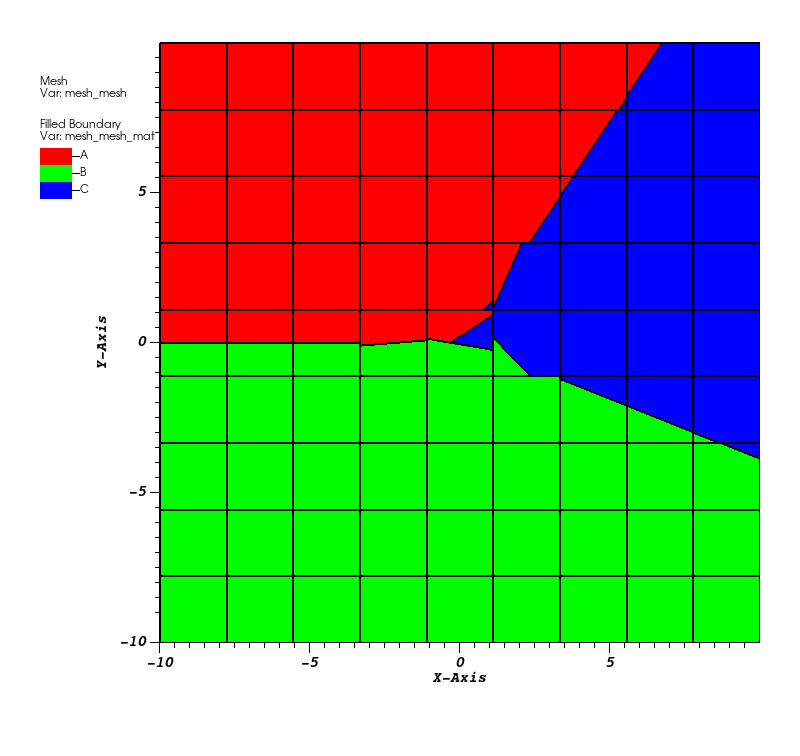
Fig. 30 Diagram showing ELVIRA MIR output from the mir_elvira2d_test application.

Example Application

The mir_concentric_circles application generates a uniform mesh with square zones, populated with circular mixed material shells. The application performs MIR on the input mesh and writes a file containing the reconstructed mesh. All program arguments (listed in the table below) are optional.

Argument	Description
–dimension number	The mesh dimension, 2 or 3.
–gridsize number	The number of zones along an axis. The default is 5.
–method name	The MIR method used “equiz” or “elvira”.
–numcircles number	The number of number of circles to use for material creation. The default is 2.
–output filepath	The file path for output files. The default is “output”.
–policy policy	Set the execution policy (seq, omp, cuda, hip)
–caliper mode	The caliper mode (none, report)

To run the example program from the Axom build directory, follow these steps:

./examples/mir_concentric_circles –gridsize 100 –numcircles 5 –output mir

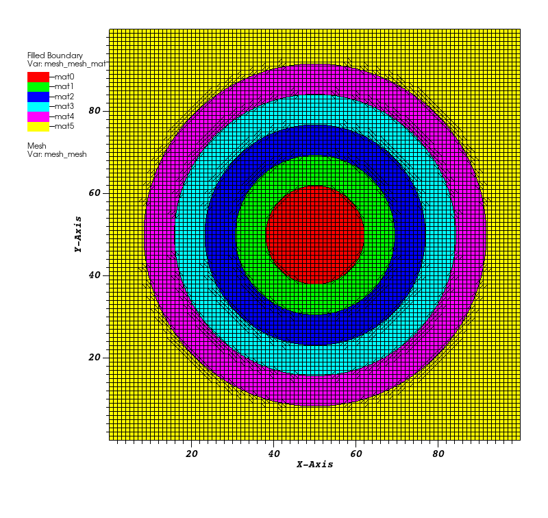
Fig. 31 Diagram showing Equi-Z MIR output from the mir_concentric_circles application.

Visualization

The VisIt software can be used to view the Blueprint output from MIR algorithms. Blueprint data is saved in an HDF5 format and the top level file has a “.root” extension. Open the “.root” file in VisIt to get started and then add a FilledBoundary plot of the material defined on the mesh topology. Plotting the mesh lines will reveal that there is a single material per zone. If the input mesh is visualized in a similar manner, zones with multiple materials will contain different colors for each material.